Introduction
The NEM is seeing a change in generation as older more conventional forms of generation retire and newer technologies such as wind, solar and storage come online. At the same time the traditional sources of primary frequency response - fast acting local responses such as those from governor action – have progressively withdrawn from the system. These changes have revealed that current frequency control mechanisms in the NEM are not “fit for purpose” and have led the Australian Energy Market Commission (AEMC) and the Australian Energy Market Operator (AEMO) to contemplate a rethink of their design.
The AEMC has recently published a final determination on the “Mandatory Primary Frequency Response” rule change proposed by AEMO. The new rule mandates a capability to provide Primary Frequency Response (PFR) to keep frequency stable within the Normal Operating Frequency Band (NOFB). This is a temporary measure as there is a sunset clause on this arrangement of 4 June 2023, after which the mandatory primary frequency response framework will be removed from the rules. The AEMC aims to replace it with a market mechanism that would promote good frequency response from participants.
IES and CS energy have been researching a mechanism that would provide a suitable financial incentive. It could overlay the currently mandated service as well as operate stand-alone. The mechanism consists of 2 parts: PFR Costing and PFR Cost Allocation. The aim of the PFR costing component is to price PFR so that it recovers an estimate of efficient costs incurred by the providers of this service. The cost allocation component aims to allocate costs and payments to participants based on performance, such that participants that cause the frequency disturbances that require PFR pay to those units that effectively provide PFR. The amount of the payment is set to the estimate of efficient cost over the settlement period.
This approach is explicitly designed to mimic as closely as possible the current regulation causer pays logic, which is familiar to NEM participants. In essence though, it is a partial implementation of the deviation pricing principles set out in the AEMC’s Frequency Control Arrangements Report and in an earlier 2017 IES Report to CS Energy on Improvements to the NEM Auction.
The remaining sections gives an overview of the two parts of the mechanism. Also outlined are some of the charts and widgets that have been made to display the results of the proposed mechanism. Access to these live charts will be given to interested parties on request.
PFR Costing
We have considered the cost of PFR to be the cost of provision by a typical thermal generator operating in a region with significant reserves in the NEM. The details of this method are provided in the next section. Some alternative approaches are outlined in a later section.
Cost of Reserve
The efficient cost of reserving capacity is calculated from the opportunity cost of reserving capacity and the capacity that should be reserved to provide PFR, offset by the reserve that is utilised. In the NEM all prices, dispatch targets and enablement levels are calculated every 5 minutes. To maintain consistency this efficient cost is also calculated for every 5-minute interval. If it were smeared over a longer period, the incentive to respond to specific (large and/or high cost) frequency events could be lost.
Opportunity Cost
The opportunity cost is defined as the unit cost of reserving capacity to provide PFR. The capacity can be in the form of headroom (for raise PFR) or footroom (for lower PFR).
This cost for a dispatch period is calculated by considering the region with the largest level of reserve (unscheduled capacity in the energy market), which is where most frequency control reserves would come from under the system-wide least cost approach that applies to other forms of FCAS. The region reference price for that region net of variable cost is calculated as the opportunity cost for that period (for the entire NEM). An example of a 24-hour period is shown below.
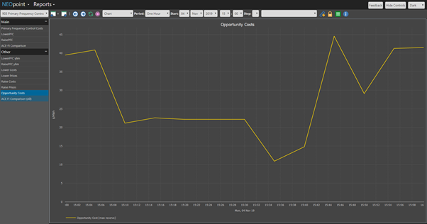
Figure 1 - Opportunity costs for a selected 1 hour period
Since a coal fired plant would likely be providing PFR (for now) we have assumed that the variable costs are that of a typical coal plant. These parameters can be easily updated.
Capacity
Capacity is a term used in this context to indicate the total MW capacity required to be reserved to provide PFR within a 5-minute dispatch interval (DI). It can be in the form of headroom (for Raise PFR) or footroom (for Lower PFR). This quantity can be calculated by considering the Area Control Error (ACE) defined for this purpose as proportional to the frequency deviation; a measure of the MW shortfall (negative) or surplus (positive). The maximum ACE (if positive) within a dispatch interval is the required headroom and the minimum ACE (if negative) is defined as the required footroom. The cost of reserving this capacity is calculated as the product of the required capacity and the opportunity cost defined above.
Note that the capacity required to be reserved is not known exactly ahead of time, so that the logic described essentially gives a lower bound of cost.
Utilisation
Any power that is utilised is paid for in the wholesale spot energy market and so should be netted off from the reserve calculated above. The negated quantity can again be calculated from the ACE. The mean over the dispatch interval of the positive quantities of ACE within a dispatch period is defined as the utilised headroom and the mean over the dispatch interval of the negative quantities of ACE within a dispatch period is defined as the utilised footroom.
An example illustrating capacity, utilisation and the net outcome for both raise and lower situations is shown in the figure following.

Figure 2 - Capacity and Utilisation values calculated from ACE
Hence the primary frequency cost (PFC) can be calculated as opportunity cost times the headroom capacity net of utilised headroom (for Raise PFC) and opportunity costs times the footroom capacity net of utilised footroom.
Raise PFC=|Opportunity Cost×(Headroom Capacity-Headroom Utilisation)|
Lower PFC=|Opportunity Cost×(Footroom Capacity-Footroom Utilisation)|
Cost Allocation
The mechanism used to allocate the costs is similar to that used to allocate FCAS costs through the Regulation Causer Pays (RCP) mechanism, a key difference being that payments are allocated to participants that provide PFR along with costs to causers.
As for RCP, costs and payments will be allocated based performance measured through AEMO’s SCADA system, which on the mainland provides data at 4 second intervals. Generation by each scheduled unit at 4 second intervals is published by AEMO daily. These data are used to quantify the performance of measured participants. This is done by comparing a unit’s measured 4second generation versus the unit’s dispatch trajectory as scheduled in the energy spot market, which is a linear between dispatch targets. The difference between the measured generation and the linear trajectory is the unit’s deviation. This is illustrated in the example below. Note that a deviation could be partly driven by the requirements of other FCAS products, including regulation[1].
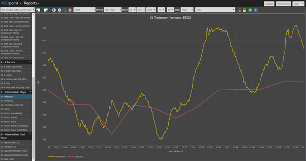
Figure 3 - Measured output (yellow) and expected trajectory (red) of a unit (ER02)
A unit’s deviation can either drive the system away from balance or toward balance. This can be determined by comparing the unit’s deviation to a quantity called ACE-REG, which is an estimate of the MW required to bring the system into balance. ACE-REG is the negative of ACE, which is an estimate of the imbalance. The unit is driving the system away from balance if the unit’s deviation is in the opposite direction of ACE-REG and is driving the system toward balance if it is in the same direction.
In Figure 3 ER02 has a significant deviation at the time around 15:40. This deviation could either be providing a balancing response for the system or an imbalancing response causing deterioration of frequency. Causation or provision can be determined from the sign of ACE-REG; positive ACE-REG implies that the system requires more generation, and vice versa. If ACE-REG is positive and deviation is positive, the unit is providing PFR. The other conditions for causer and provider are given in the table 1 below. Figure 4 identifies regions of causation and provision by colour coding deviation and ACE-REG by sign.
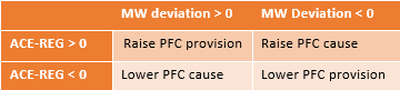
Table 1 - Provider, Causer relations
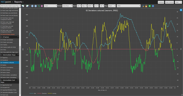
Figure 4 - Colour coded chart of deviation vs ACE-REG: yellow:positive ACE-REG green:negative ACE-REG blue:positive deviation red:negative deviation (ER02)
The scale of the causation or provision depends on the relative magnitudes of the unit’s deviation and ACE-REG. This can be further quantified by the product of the 2 quantities (labelled the unit’s 4-second performance factor); a positive factor implies that the unit is providing power to reduce frequency deviation for that 4sec interval while a negative factor implies that the unit is causing an further imbalance in that interval. ER02’s performance factors for the selected period are given in figure 5. Notice the peaks between 15:35 to 15:45, they coincide with periods of high ACE-REG (both positive and negative)
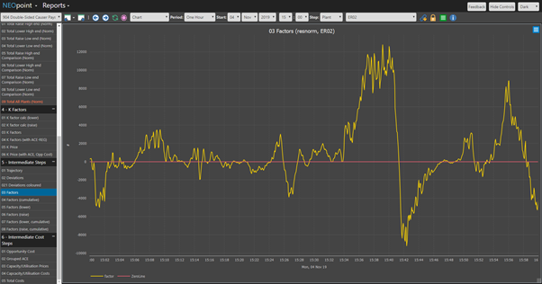
Figure 5 - Plot of performance factors (ER02)
These factors are then aggregated into four separate 5-minute buckets; two for Raise (causer and provider) and two for Lower (causer and provider). i.e. a unit can be a causer and a provider for both Raise and Lower within a single 5-minute period, but at different scales.
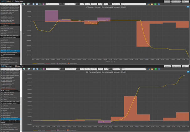
Figure 6 - Top: Lower 5min factors (provider: orange, causer: purple) and cumulative lower 4sec performance factors (yellow), bottom: Raise 5min factors and cumulative raise 4sec performance factors (for ER02)
The factors can be used as weighting factors to allocate cost to both causers and providers. A representation of the costs/payments allocated to ER02 based on this 1-hour period is provided in figure 7. Under this mechanism a unit can have both causer and provider allocations (for both Raise and Lower) within a single dispatch period.
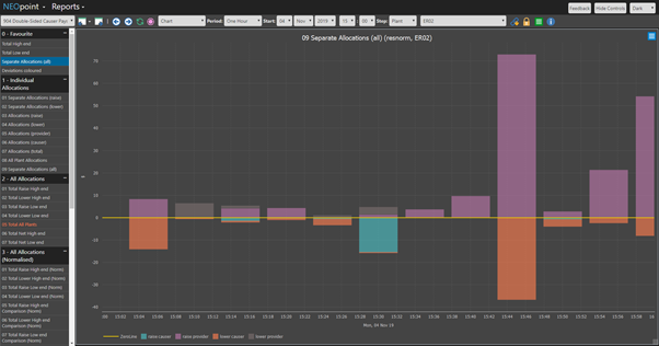
Figure 7 - All costs/payments allocated to ER02 (purple: Raise Provision, orange: Lower Causation, grey: Lower Provision, blue: Raise Causation)
Other Approaches to Costing
The cost allocation mechanism described above does not depend on how the efficient PFR cost is calculated. A completely different cost estimate could be used to allocate costs.
One approach would be to follow the approach of RCP and simply use the sum of the raw factors for payment and cost allocation purposes. Such an approach provides different incentives to perform depending on market conditions, a flaw shared with RCP. Nevertheless, it has the virtue of simplicity, so we have provided some plots of accumulated factors in our charting suite.
AEMO in its submissions to AEMC has been trumpeting the virtues of encouraging a wide geographic spread of PFR. This could be encouraged by weighting performance factors by the local spot market price at each connection point. The cost may be a little higher but the technical result superior. Weighting by the local spot market price also offers the prospect of much easier hedging against the cost of the service.
Other Issues
In this article we have not addressed a range of important policy issues that would need to be resolved to implement a scheme along the lines described. For example, what is the relationship between RCP and the PFR payment mechanism described in this article? In essence, they operate on different timescales. Is there a problem with double payment for PFR and for regulation enablement? Should there be a lag between measurement and payment to mimic RCP? These are questions that need examination based on economic and control theory and practice.
Results
Charts
A range of charts illustrating the calculation process and presenting results are accessible from NEOpoint. The details of each chart are beyond the scope of this article. Please contact us if you would like further information. A general overview of each section is provided below.
903 – Primary Frequency Control Costs
Displays charts relating to calculating the efficient cost of PFR.
904 - Double Sided Causer Pays
Displays charts relating to the cost allocation process. A breakdown of each section is provided below.
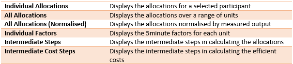
Table 2 - Section overview of 904 Double Sided Causer Pays
It should be noted that this mechanism is not yet implemented so no units are responding to this incentive. The data displayed in these charts could be significantly different if units were responding to this incentive.
For practical reasons we are not able to store results for all times; The charts in “Intermediate Steps” for example which requires very high-resolution data will only display results for the periods laid out in table 3. The remaining sections contain data at 5-minute resolution which can be stored more easily, hence the remaining section will be able to display results from at least 1 Jan 2020. New results are published as AEMO publishes the associated 4 second data.

Table 3 - Available periods for high-resolution data
Charts displaying 4 second data (with 4s in the title) can take a long time to complete if selected to run over more than a few hours. Accordingly, the chart will not run if a run period over "three hours" is selected. This will be displayed in the log. Select a period of 3 hours or less to run these charts. If you need to see an outcome over a longer period such as a settlement period, use the 5 minute data (not labelled as 4s).
Note: If you have any questions or you cannot access the charts please get in touch via the contact details in the right navigation bar.
1 This raises the issue of whether operating under different overlapping services or arrangements constitute inappropriate double counting. This document does not address this or several other policy issues. However, we would argue that markets will adjust to overlapping services and so there is no practical problem.
IES provides expert advice and powerful tools for electricity and gas market.
+61 2 9436 2555info@iesys.com
www.iesys.com
© 2025 Intelligent Energy Systems. All Rights Reserved.